The purpose of this tutorial is to illustrate R best practices that facilitate efficient Shiny app development and debugging. All of these best practices pertain to writing R code in general beyond Shiny apps. We bring them up as part of the Shiny course because Shiny apps have many moving parts. Keeping our code as human-readable, automated, and compartmentalized as possible will help us spend less of our time debugging and more of our time communicating science.
Before we begin
If we’re going to chat about a dry subject like optimizing code, we might as well have a little fun. If you want to code along with this tutorial, you’ll need the wingspan package, which contains data from the delightful wingspan board game, wherein you win points through various bird-related challenges. We’ll also need the colorblinr package for some accessibility testing and the remotes package to install wingspan and colorblindr from github. In addition, we’ll need the tidyverse package, so go ahead and install that too if you haven’t already.
Naming conventions
When choosing names for data, we have to balance the needs to be concise, descriptive, and consistent. Let’s assume we want to make two dataframes, one containing information on platform-nesting birds, and one containing information on cavity-nesting birds. We could name our two dataframes Data1 and data_2.
We’ll create our dataframes using the filter() function from the dplyr package, which comes as a part of the tidyverse. filter() keeps only rows that match the conditions in the parentheses, here that nest_type equals “Platform” and “Cavity,” respectively. The %>% is called a “pipe,” and it essentially means “take everything from the left side of the pipe and apply this series of operations to it.” It saves us from having to make a new data frame each time we want to apply a new function or calculation.
birds <- wingspan::birds


Data1 <- birds %>% filter(nest_type == "Platform")
data_2 <- birds %>% filter(nest_type == "Cavity")

Data1[1:5, 1:5]
# A tibble: 5 x 5
  common_name    scientific_name    set    power_color power_category
  <chr>          <chr>              <chr>  <chr>       <chr>
1 Abbott's Booby Papasula abbotti   ocean~ White       <NA>
2 American Bitt~ Botaurus lentigin~ core   Brown       Card-drawing
3 American Coot  Fulica americana   core   Brown       Flocking
4 American Crow  Corvus brachyrhyn~ core   Brown       Food from Supp~
5 Anhinga        Anhinga anhinga    core   Brown       Hunting/Fishing
These names are concise and they work just fine from the computer’s perspective. However, it will be easier for us as humans to organize our code and our thoughts if our data structures and modeling components follow one framework for naming. Some popular frameworks include camelCase/CamelCase where we use capital letters to mark breaks between words or snake_case where we use underscores to separate words. Since we’re focusing on human readability, you should go with whatever format works for you as long as you use it to build a consistent naming convention. The Advanced R book suggests using lower-case nouns for variables and dataframes, so that’s what we’ll do here:
Now our names are concise and follow a similar style, but they’re not terribly descriptive. This might be fine if we just have one or two dataframes, but having lots of similarly-named dataframes can make it hard for us to keep our data straight later when we start building more complex data structures or when we hand off the project to someone else. Let’s give our dataframes some more descriptive names reflecting their content:
Comments
At this point, our code making a dataframe of platform-nesting bird data and a dataframe of cavity-nesting bird data is nice and clear. To us. Today. But what if we want to share it with someone who didn’t get our lovely introduction above? Or what if we need to put it down for a few months (life happens) and pick it up later?
One of the kindest things we can do for ourselves is to liberally annotate our code with comments. A good comment can accomplish many things. It can include useful metadata and information on the code developers. Crucially, comments also give us a way to track dependencies, changes, and developments in our code so we can save time debugging when things go wrong later. Especially important to us as scientists, we can use comments to record our objectives and explain how our code meets them.
# Make a dataframe of platform nesters and a dataframe of cavity nesters
# using the birds data from the wingspan package and the filter()
# function from the dplyr package.
birds <- wingspan::birds
platform_nesters <- birds %>% filter(nest_type == "Platform")
cavity_nesters <- birds %>% filter(nest_type == "Cavity")
Text wrapping and visual layouts
In addition to supplementing our code with abundant, descriptive comments, we can make our coding lives much easier with some strategic text wrapping and visual layouts. One of the nice things about R is that we can arrange our code with line breaks and spacing to make it easy to read and scan for mistakes. Let’s update our code using the select() function from the dplyr package to select several columns. If we keep everything on one line like we did above, it quickly gets overwhelming (note our new comment reflecting our update!):
# Make a dataframe of platform nesters and a dataframe of cavity nesters
# using the birds data from the wingspan package and the filter()
# function from the dplyr package.

# Update: added select function to select several columns
birds <- wingspan::birds
platform_nesters <- birds %>% filter(nest_type == "Platform") %>% select(common_name, scientific_name, nest_type, egg_capacity, wingspan, forest, grassland, wetland, invertebrate, seed, fish, fruit, rodent, nectar, any_food)
cavity_nesters <- birds %>% filter(nest_type == "Cavity")%>% select(common_name, scientific_name, nest_type, egg_capacity, wingspan, forest, grassland, wetland, invertebrate, seed, fish, fruit, rodent, nectar, any_food)

platform_nesters[1:5, 1:5]
# A tibble: 5 x 5
  common_name      scientific_name     nest_type egg_capacity wingspan
  <chr>            <chr>               <chr>            <dbl>    <dbl>
1 Abbott's Booby   Papasula abbotti    Platform             1      190
2 American Bittern Botaurus lentigino~ Platform             2      107
3 American Coot    Fulica americana    Platform             5       61
4 American Crow    Corvus brachyrhync~ Platform             2       99
5 Anhinga          Anhinga anhinga     Platform             2      114
Breaking up our code over several lines at the pipes %>% and commas between selected columns gives us a much cleaner code block that’s easier to navigate. Advanced R recommends limiting lines to 80 characters or fewer as a rule of thumb. From here forward, we’ll use the platform_nesters and cavity_nesters dataframes and add on to them.
# Make a dataframe of platform nesters and a dataframe of cavity nesters
# using the birds data from the wingspan package and the filter()
# function from the dplyr package.

# Update: added select function to select several columns

birds <- wingspan::birds

platform_nesters <- birds %>%
                    filter(nest_type == "Platform") %>%
                    select(common_name,
                           scientific_name,
                           nest_type,
                           egg_capacity,
                           wingspan,
                           forest,
                           grassland,
                           wetland,
                           invertebrate,
                           seed,
                           fish,
                           fruit,
                           rodent,
                           nectar,
                           any_food)


cavity_nesters <- birds %>%
                  filter(nest_type == "Cavity")%>%
                  select(common_name,
                         scientific_name,
                         nest_type,
                         egg_capacity,
                         wingspan,
                         forest,
                         grassland,
                         wetland,
                         invertebrate,
                         seed,
                         fish,
                         fruit,
                         rodent,
                         nectar,
                         any_food)
Functions
As soon as we progress beyond very basic operations in R, we’ll find ourselves having to do the same operation multiple times. Functions allow us to automate these kinds of repetitive tasks. Let’s say we really want to win at wingspan by collecting the most eggs possible. Given that food is a limited resource in the game, we might want to play the birds with the highest return of eggs per unit food item. We can update our code blocks to give us only birds above a critical efficiency threshold, let’s say 3 eggs per food item. We won’t save our observations just yet. Instead, we’ll select a few columns to look at and just print the dataframes.
              platform_nesters %>%
                    mutate(egg_efficiency = # calculate return of eggs/ unit food
                           egg_capacity/
                           (seed + fish +
                            fruit + rodent +
                            nectar + any_food)) %>%
                    arrange(desc(egg_efficiency)) %>% # arrange in descending order
                    select(common_name, egg_efficiency) %>%
                    filter(egg_efficiency >= 3) # keep only birds with efficiency >= 3
# A tibble: 10 x 2
   common_name           egg_efficiency
   <chr>                          <dbl>
 1 Griffon Vulture                  Inf
 2 Mourning Dove                      5
 3 Ruddy Duck                         5
 4 Crested Pigeon                     4
 5 Peaceful Dove                      4
 6 Pied-Billed Grebe                  4
 7 Common Little Bittern              3
 8 Eurasian Magpie                    3
 9 Green Heron                        3
10 King Rail                          3
cavity_nesters %>%
mutate(egg_efficiency = # calculate return of eggs/ unit food
egg_capacity/
(seed + fish +
fruit + rodent +
nectar + any_food)) %>%
arrange(desc(egg_efficiency)) %>% # arrange in descending order
select(common_name, egg_efficiency) %>%
filter(egg_efficiency >= 3) # keep only birds with efficiency >= 3
# A tibble: 39 x 2
   common_name          egg_efficiency
   <chr>                         <dbl>
 1 Black Vulture                   Inf
 2 Common Swift                    Inf
 3 European Bee-Eater              Inf
 4 House Wren                      Inf
 5 Purple Martin                   Inf
 6 Turkey Vulture                  Inf
 7 Vaux's Swift                    Inf
 8 Violet-Green Swallow            Inf
 9 White-Throated Swift            Inf
10 Coal Tit                          6
# ... with 29 more rows
Again, this works fine. BUT, there’s no reason for us to do the same work twice. Instead, let’s write a function that lets us calculate egg efficiency and retain only birds with egg efficiency above a threshold. This will work exactly like any other R function like mean() etc. We just have to write out our summary code as we did above, substituting flexible argument names, and then run the function in the console. This is called “sourcing.” When we source a function, it should appear in our environment pane. Once we source our new function, called calc_egg_eff, using lower-case verbs as suggested by Advanced R, we’ll just print the dataframes to inspect them rather than saving them to new objects.
# Writing a function to calculate egg efficiency and keep only birds above a critical
# egg efficiency value

calc_egg_eff <- function(bird_df, # function arguments with no defaults. Bird dataframe
                         egg_threshold){ # work just like any other function. Critical egg threshold.


  bird_df <- bird_df %>%
             mutate(egg_efficiency = # calculate return of eggs/ unit food
                    egg_capacity/
                    (seed + fish +
                     fruit + rodent +
                     nectar + any_food)) %>%
                     arrange(desc(egg_efficiency)) %>% # arrange in descending order
                     select(common_name, egg_efficiency) %>%
                     filter(egg_efficiency >= egg_threshold)

  # what to return when the function is called.

  return(bird_df)

  }

# make a summary dataframe of platform nesters including only birds with egg efficiency greater than 3.

          calc_egg_eff(bird_df = platform_nesters,
                       egg_threshold = 3)  # keep only birds with efficiency >= 3
# A tibble: 10 x 2
   common_name           egg_efficiency
   <chr>                          <dbl>
 1 Griffon Vulture                  Inf
 2 Mourning Dove                      5
 3 Ruddy Duck                         5
 4 Crested Pigeon                     4
 5 Peaceful Dove                      4
 6 Pied-Billed Grebe                  4
 7 Common Little Bittern              3
 8 Eurasian Magpie                    3
 9 Green Heron                        3
10 King Rail                          3
# And make a summary dataframe for cavity nesters
calc_egg_eff(bird_df = cavity_nesters,
egg_threshold = 3)
# A tibble: 39 x 2
   common_name          egg_efficiency
   <chr>                         <dbl>
 1 Black Vulture                   Inf
 2 Common Swift                    Inf
 3 European Bee-Eater              Inf
 4 House Wren                      Inf
 5 Purple Martin                   Inf
 6 Turkey Vulture                  Inf
 7 Vaux's Swift                    Inf
 8 Violet-Green Swallow            Inf
 9 White-Throated Swift            Inf
10 Coal Tit                          6
# ... with 29 more rows
Much cleaner! If you want to take developing your own functions a step further (your should!), you can write all your functions in a seperate script and source it or write your own R package. It’s easier than you might expect!. For right now, we’ll just write ourselves one egg efficiency function and appreciate our cleaned-up code.
Accessibility
Best practices for R graphics take up entire books. We’re just going to touch briefly on graphics here to provide some guidance for accessibility. Specifically, we’ll deal with making graphics color-blind safe. We’ll talk more about accessibility in the Shiny-specific Best Practices section.
First, let’s address colors. Color can be an important tool for data visualization, but we need to make sure our great colors are actually interpretable to everyone. Colors are composed of hues (the slice of the color wheel a color occupies) and value (the ammount of black in the color). By choosing colors that contrast values as well as hues, we can make sure that color-blind audience members can interpret our visuals. To see the impact of using hues and values strategically in practice, let’s make a plot of some of our wingspan data using the ggplot package. Using ggplot(), we’ll make a scatter plot with birds’ wingspan on the x axis and victory points on the y axis, with color determined by whether or not a bird is a predator via the scale_color_manual() function.
# Make a scatter plot called victory_point
# displaying wingspan on the x axis and victory points on the y axis
# Make non-predators dark red and predators green

victory_plot <- ggplot(birds) +
                 geom_point(aes(x = wingspan,
                                y = victory_points,
                                color = predator),
                            size = 3) +
                 scale_color_manual(values = c("FALSE" = "darkred",
                                    "TRUE" = "darkgreen")) +
                 theme_bw()

# print victory_plot

victory_plot
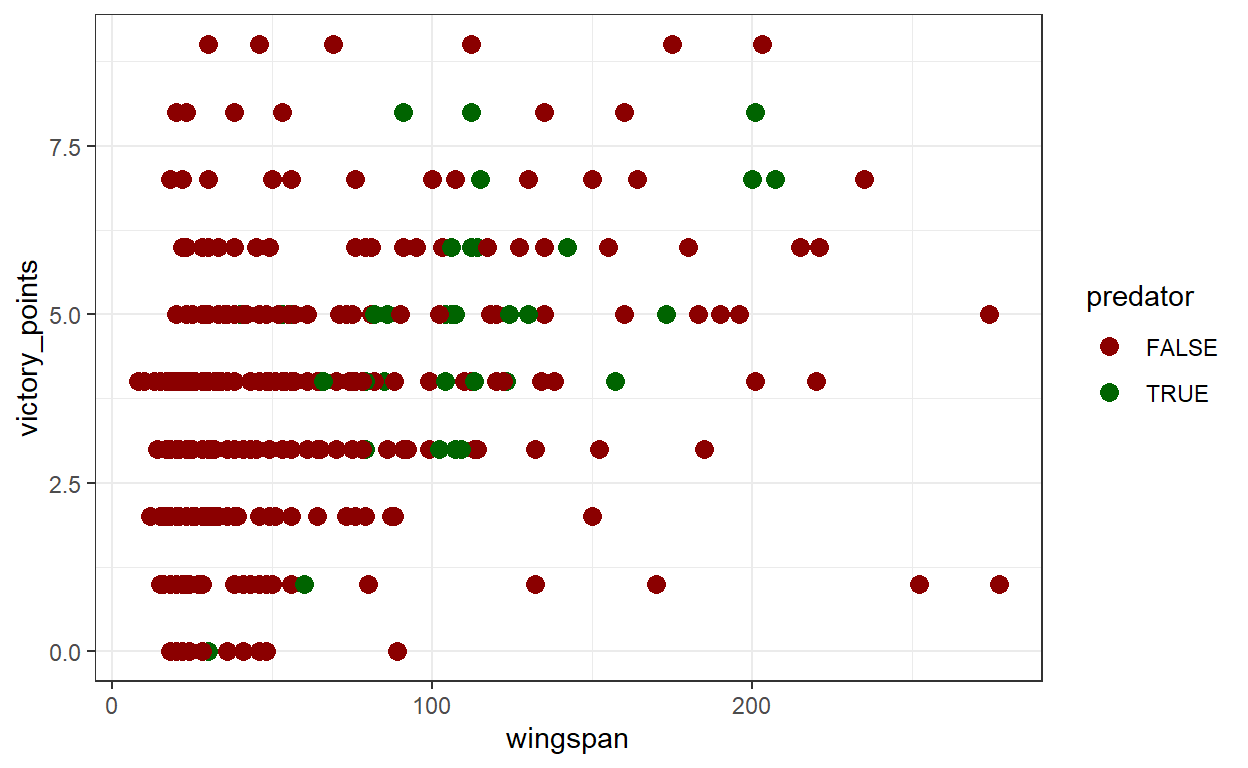
Assuming you’re not colorblind, this plot looks ok. Now we’ll use the cvd_grid() function from the colorblindr package to simulate what the plot would look like to people with different forms of colorblindness.
# Simulate what victory_plot would look like to people with different
# kinds of color blindness.

cvd_grid(victory_plot)
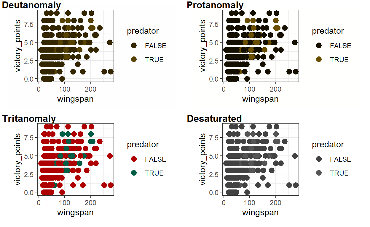
# Hard to distinguish between predators and non-predators.
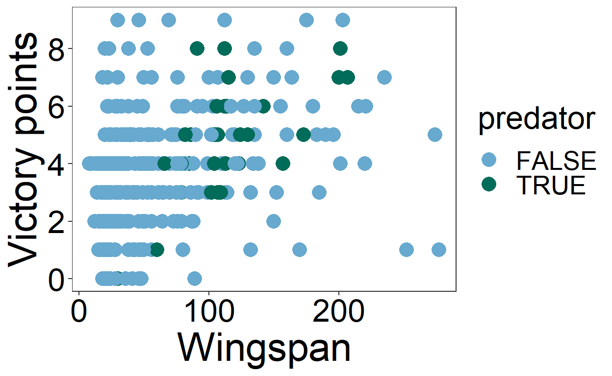
It’s much harder to distinguish the difference between predators and non-predators! That’s because even though the darkred and darkgreen colors have different hues, they have similar values. Let’s try distinguishing between predators and non-predators using colors that differ in value as well as hue. We’ll also make the text bigger and visually simplify the plot by removing the panel lines and adjusting the y scale (the last two are more preferences than accessibility issues). We’ll call our revised plot victory_plot_cbf for “colorblind friendly.”
# Make a scatter plot called victory_point
# displaying wingspan on the x axis and victory points on the y axis
# Make non-predators light blue and predators dark green
victory_plot_cbf <- ggplot(birds) +
geom_point(aes(x = wingspan,
y = victory_points,
color = predator),
size = 5) +
scale_color_manual(values = c("FALSE" = "#67a9cf",
"TRUE" = "#016c59")) +
labs (x = "Wingspan", y = "Victory points") +
scale_y_continuous(breaks = seq(0, 8, 2)) +
theme_bw() +
theme(axis.text = element_text(size = 24,
color = "black"),
axis.title = element_text(size = 36),
panel.grid = element_blank(),
legend.title = element_text(size = 24),
legend.text = element_text(size = 20))
# print victory_plot
victory_plot_cbf
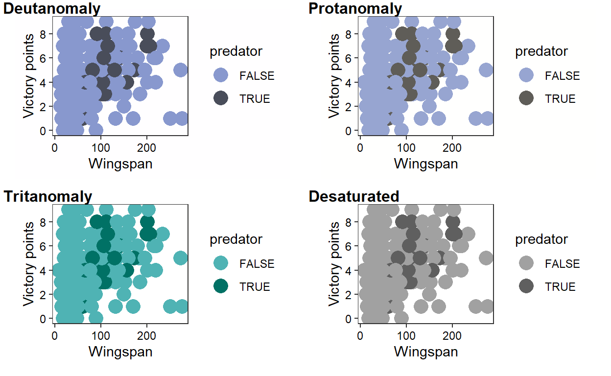
# Simulate what victory_plot would look like to people with different
# kinds of color blindness.
cvd_grid(victory_plot_cbf)
# Much more colorblind friendly!
# Make a scatter plot called victory_point
# displaying wingspan on the x axis and victory points on the y axis
# Make non-predators light blue and predators dark green

victory_plot_cbf <- ggplot(birds) +
                     geom_point(aes(x = wingspan,
                                    y = victory_points,
                                    color = predator),
                                    size = 5) +
                     scale_color_manual(values = c("FALSE" = "#67a9cf",
                                        "TRUE" = "#016c59")) +
                     labs (x = "Wingspan", y = "Victory points") +
                     scale_y_continuous(breaks = seq(0, 8, 2)) +
                     theme_bw() +
                     theme(axis.text = element_text(color = "black"),
                           panel.grid = element_blank())

# print victory_plot

victory_plot_cbf +
       theme(axis.text = element_text(size = 24,
             color = "black"),
             axis.title = element_text(size = 30),
             panel.grid = element_blank(),
             legend.title = element_text(size = 24),
             legend.text = element_text(size = 20))
# Simulate what victory_plot would look like to people with different
# kinds of color blindness.

cvd_grid(victory_plot_cbf)
# Much more colorblind friendly!
Our revised plot is much easier to interpret! We retain contrast when we simulate what our plot would look like to people with different kinds of color-blindness. If you want to try different combinations of colorblind-friendly colors, check out color brewer
Next Steps
These best practices are based on the Advanced R book and R for Data Science books. If you want to learn more about best practices from expert software engineers, I would absolutely check out those books, as well as recorded talks from conferences like UseR and Rstudio::conf.
Article by Lyndsie Wszola